Presenter #1 |
James L. Green, Director
Planetary Science Division, NASA Headquarters, Washington, D.C.
|
Presenter #2 |
Sean C. Solomon, MESSENGER Principal Investigator
Lamont-Doherty Earth Observatory, Columbia University, Palisades, N.Y.
Image 2.1

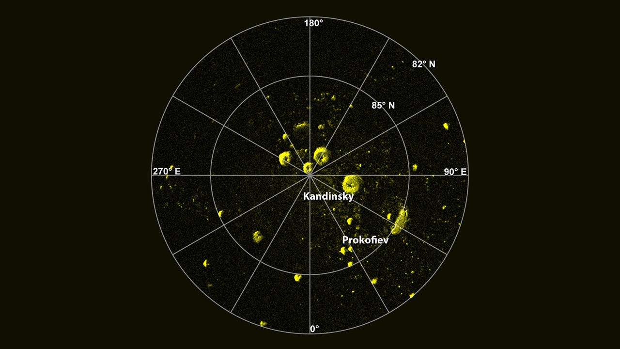
A radar image of Mercury’s north polar region acquired by the Arecibo Observatory. Yellow areas denote regions of high radar reflectivity. Since their discovery in 1992, these polar deposits have been hypothesized to consist of water ice trapped in permanently shadowed areas near Mercury's north and south pole, but other explanations for the polar deposits have also been suggested. Polar stereographic projection. From J. K. Harmon et al., Icarus, 211, 37–50 (2011).
Credit: National Astronomy and Ionosphere Center, Arecibo Observatory.
Click on image to enlarge.
Download image for print.
|
|
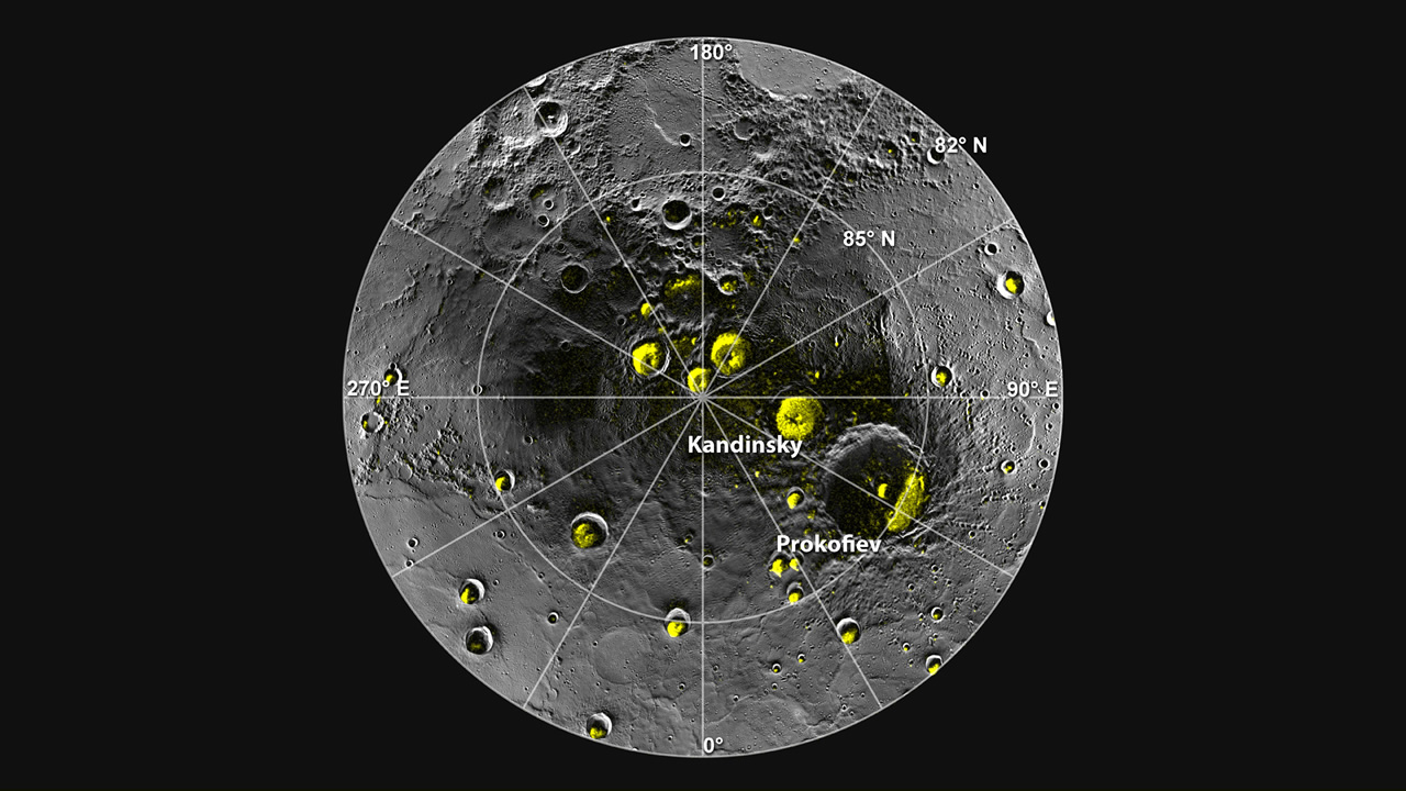
Image 2.2

The radar image of Mercury’s north polar region from Image 2.1 is shown superposed on a mosaic of MESSENGER images of the same area. All of the larger polar deposits are located on the floors or walls of impact craters. Deposits farther from the pole are seen to be concentrated on the north-facing sides of craters. Updated from N. L. Chabot et al., Journal of Geophysical Research, 117, doi: 10.1029/2012JE004172 (2012).
Credit: NASA/Johns Hopkins University Applied Physics Laboratory/Carnegie Institution of Washington/National Astronomy and Ionosphere Center, Arecibo Observatory
Click on image to enlarge.
Download image for print.
|
|
Image 2.3

Shown in red are areas of Mercury’s north polar region that are in shadow in all images acquired by MESSENGER to date. Image coverage, and mapping of shadows, is incomplete near the pole. The polar deposits imaged by Earth-based radar are in yellow (from Image 2.1), and the background image is the mosaic of MESSENGER images from Image 2.2. This comparison indicates that all of the polar deposits imaged by Earth-based radar are located in areas of persistent shadow as documented by MESSENGER images. Updated from N. L. Chabot et al., Journal of Geophysical Research, 117, doi: 10.1029/2012JE004172 (2012).
Credit: NASA/Johns Hopkins University Applied Physics Laboratory/Carnegie Institution of Washington/National Astronomy and Ionosphere Center, Arecibo Observatory
Click on image to enlarge.
Download image for print.
|
|
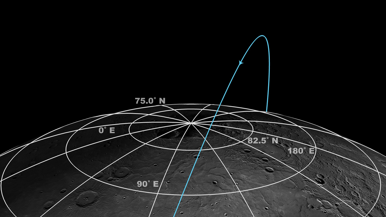
Image 2.4

This schematic of MESSENGER’s orbit illustrates some of the challenges to acquiring observations of Mercury’s north polar region. During its primary orbital mission, MESSENGER was in a 12-hour orbit and was at an altitude between 244 and 640 km at the northernmost point in its trajectory. Since April 2012, MESSENGER has been in an 8-hour orbit (shown here), and it has been at an altitude between 311 and 442 km at the northernmost point in its trajectory. Even from these high-latitude vantages, Mercury’s polar deposits fill only a small portion of the field of view of many of MESSENGER’s instruments.
Credit: NASA/Johns Hopkins University Applied Physics Laboratory/Carnegie Institution of Washington
Click on image to enlarge.
|
|
Presenter #3 |
David J. Lawrence, MESSENGER Participating Scientist
The Johns Hopkins University Applied Physics Laboratory, Laurel, Md.
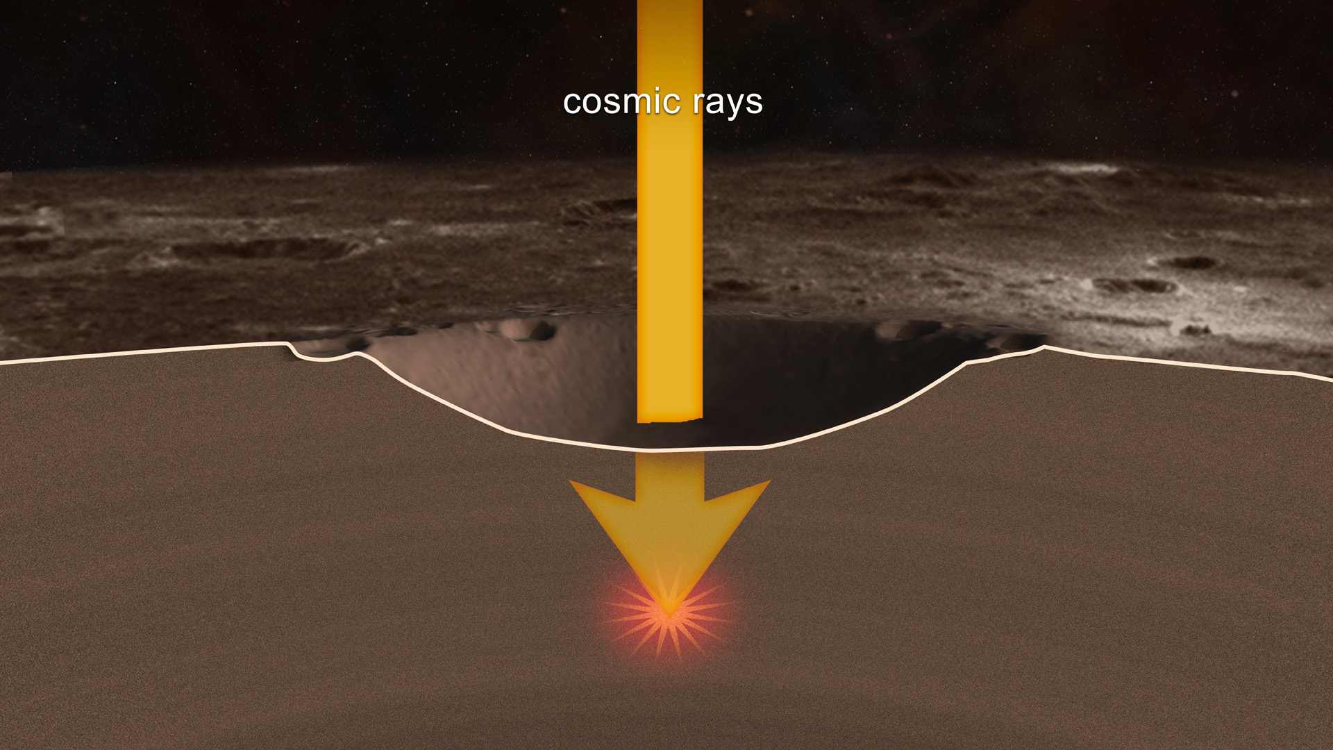
Image 3.1a

Image 3.1b

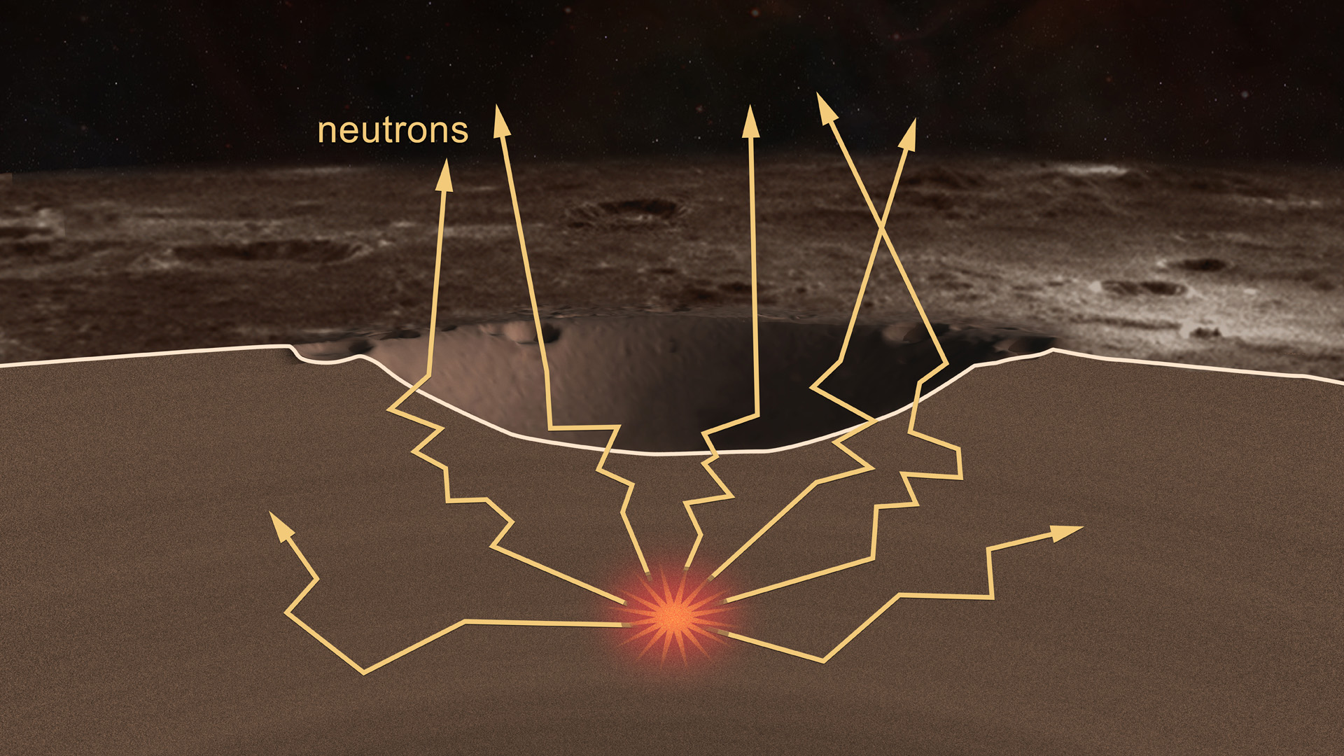
MESSENGER uses neutron spectroscopy to measure average hydrogen concentrations within Mercury’s radar-bright regions. Water ice concentrations are derived from the hydrogen measurements. When a galactic cosmic ray (thick yellow arrow) strikes Mercury, it liberates neutrons (thin arrows) from atomic nuclei in Mercury’s near-surface material. The neutrons travel multiple meters through the surface and escape into space, where some can be detected by the Neutron Spectrometer on the orbiting MESSENGER spacecraft.
Credit: NASA/Johns Hopkins University Applied Physics Laboratory/Carnegie Institution of Washington
Click on image to enlarge.
|
Image 3.1c

A layer of water ice several meters thick is illustrated in white. Abundant hydrogen atoms within the ice stop the neutrons from escaping into space. A signature of enhanced hydrogen concentrations (and, by inference, water ice) is a decrease in the rate of MESSENGER’s detection of neutrons from the planet.
Credit: NASA/Johns Hopkins University Applied Physics Laboratory/Carnegie Institution of Washington
Click on image to enlarge.
|
|
Image 3.2a

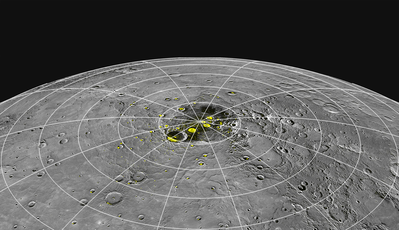
Perspective view of Mercury’s north polar region with the radar-bright regions shown in yellow.
Credit: NASA/Johns Hopkins University Applied Physics Laboratory/Carnegie Institution of Washington
Click on image to enlarge.
|
Image 3.2b

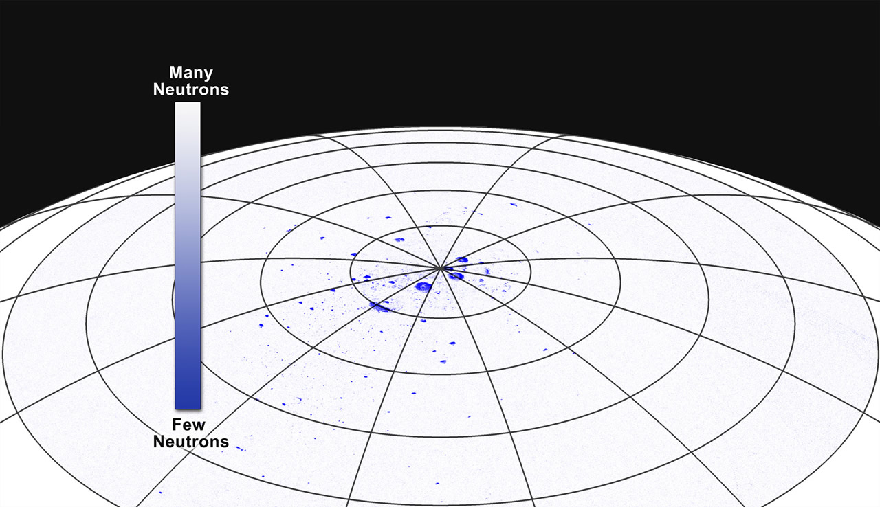
Mercury’s north polar region if viewed by a neutron spectrometer with perfect focus. Measurements over radar-bright regions that consist of pure water ice would show fewer neutrons per given time interval than elsewhere.
Credit: NASA/Johns Hopkins University Applied Physics Laboratory/Carnegie Institution of Washington
Click on image to enlarge.
|
Image 3.2c

The focus of MESSENGER’s Neutron Spectrometer is blurred by spacecraft altitude and the fact that neutrons enter the detector from many directions. Measured neutrons will show a decreased flux near the poles if water ice dominates the material in all the radar-bright regions.
Credit: NASA/Johns Hopkins University Applied Physics Laboratory/Carnegie Institution of Washington
Click on image to enlarge.
|
|
Image 3.3a

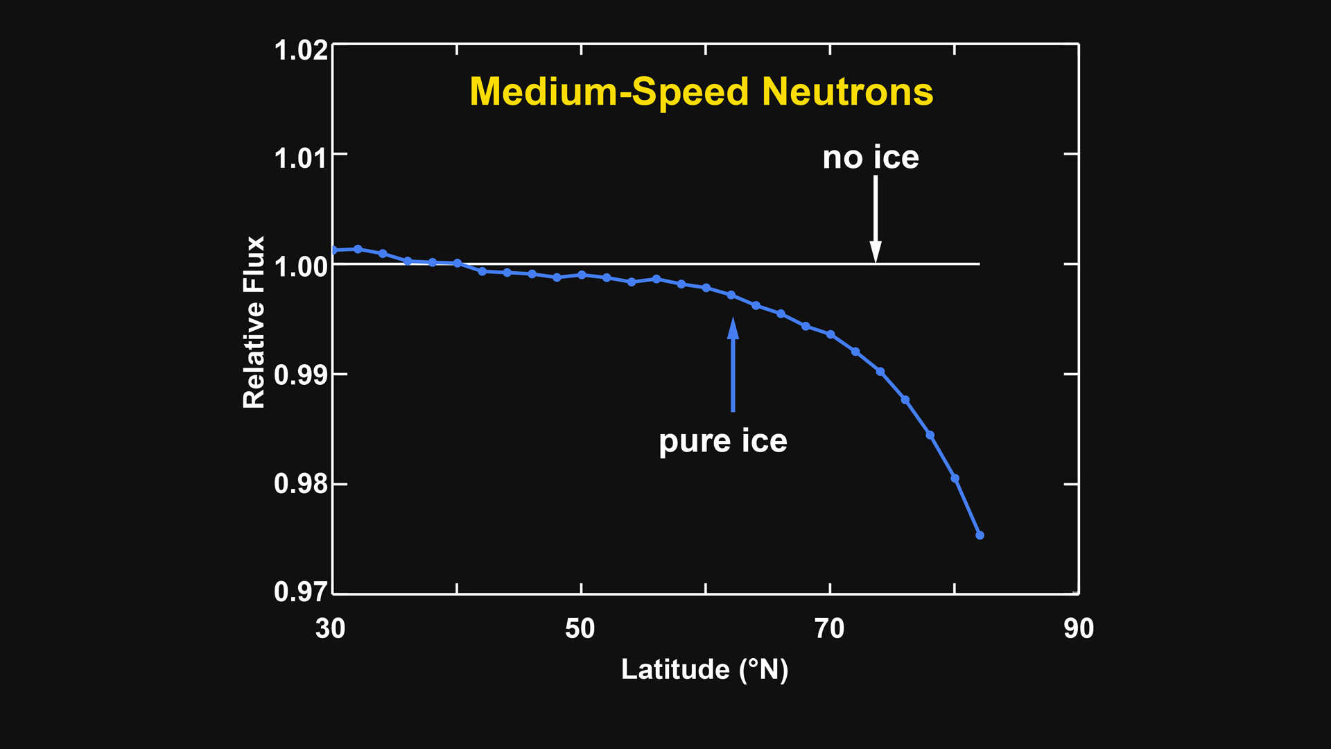
Simulated variations of medium-speed (or epithermal) neutrons with latitude are shown under two hypotheses: (1) there is no ice in the radar-bright regions; and (2) all radar-bright regions consist of a thick layer of pure water ice. The vertical axis shows the relative neutron flux (or relative number of neutrons per given time), the horizontal axis shows latitude, and the north pole is at the right at 90º latitude. If the radar-bright regions have little to no water ice, the neutron flux will show no change with latitude (white line). If the radar-bright regions consist of pure water ice, the neutron flux will show a decrease toward the north pole (blue line).
Credit: NASA/Johns Hopkins University Applied Physics Laboratory/Carnegie Institution of Washington
Click on image to enlarge.
|
Image 3.3b

MESSENGER Neutron Spectrometer measurements of the flux of medium-speed neutrons versus latitude are shown in red. The data closely match the simulation with pure water ice within Mercury’s radar-bright areas. These data demonstrate that Mercury’s polar regions have enhanced hydrogen at concentrations consistent with pure ice in the polar deposits.
Credit: NASA/Johns Hopkins University Applied Physics Laboratory/Carnegie Institution of Washington
Click on image to enlarge.
|
Image 3.3c

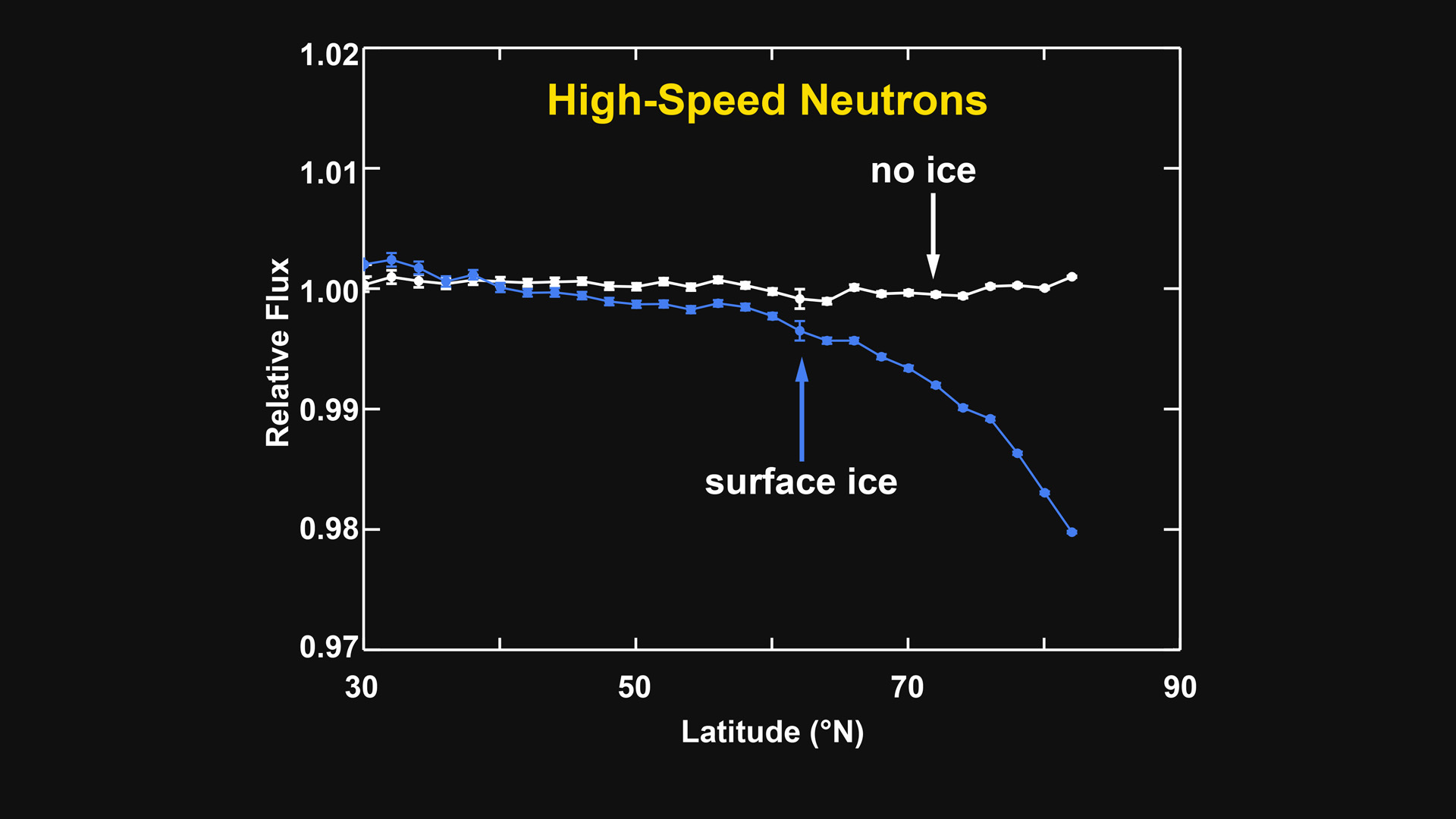
High-speed (or fast) neutrons complement the medium-speed neutrons by providing a measure of the burial depth of a thick layer of water ice beneath a thinner surface layer of material with less hydrogen. Simulated variations of high-speed neutrons are shown for two hypotheses: (1) there is no ice in the radar-bright regions; and (2) all radar-bright regions consist of a thick layer of pure water ice at the surface. If the radar-bright regions have little to no water ice, the neutrons will show no change with latitude (white line). If the radar-bright regions consist of pure water ice at the surface, the neutron flux will show a decrease toward the north pole (blue line).
Credit: NASA/Johns Hopkins University Applied Physics Laboratory/Carnegie Institution of Washington
Click on image to enlarge.
|
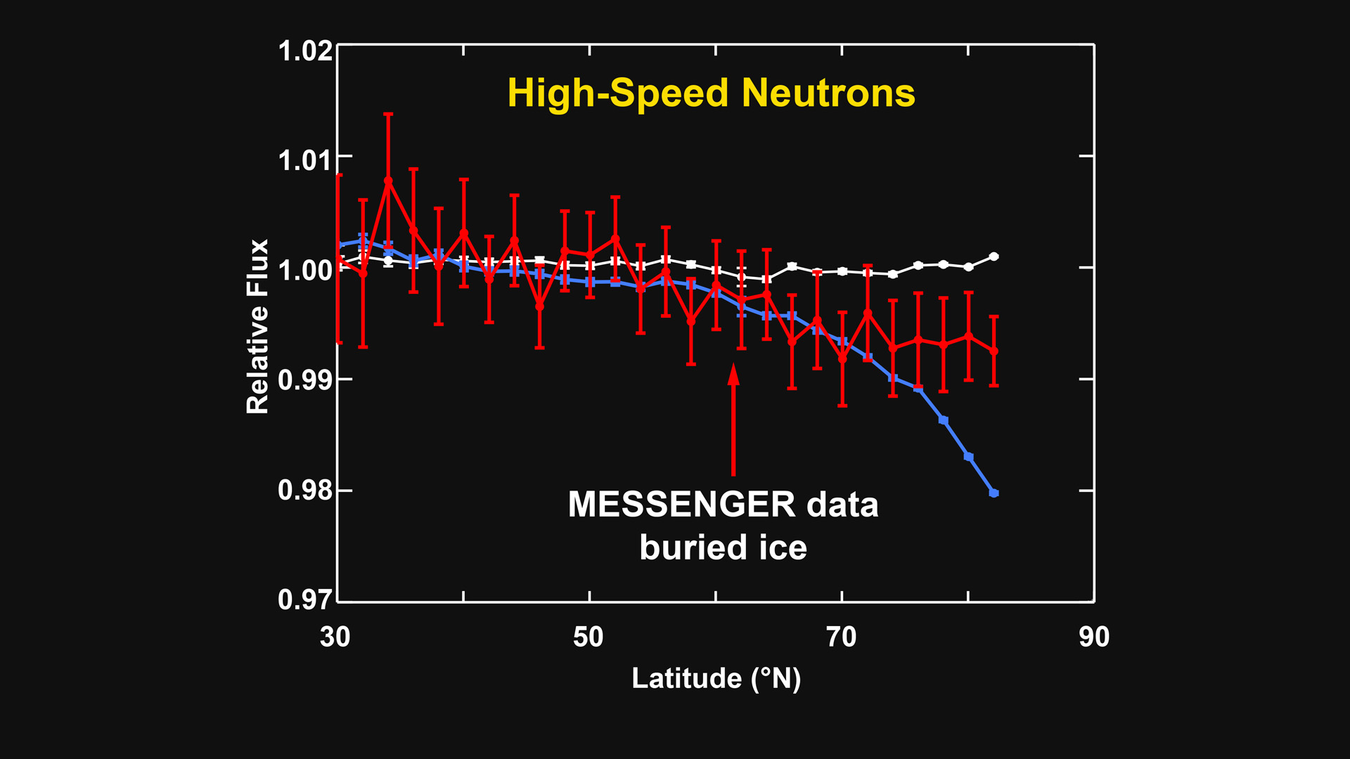
Image 3.3d

High-speed (or fast) MESSENGER Neutron Spectrometer measurements of the flux of high-speed neutrons versus latitude are shown in red. The decrease in neutron flux toward the north pole is smaller than expected if water ice were at the surface in all radar-bright areas. Therefore, high-speed neutrons indicate that most of the water ice is buried, on average, by a layer of low-hydrogen material 10 to 20 cm thick.
Credit: NASA/Johns Hopkins University Applied Physics Laboratory/Carnegie Institution of Washington
Click on image to enlarge.
|
|
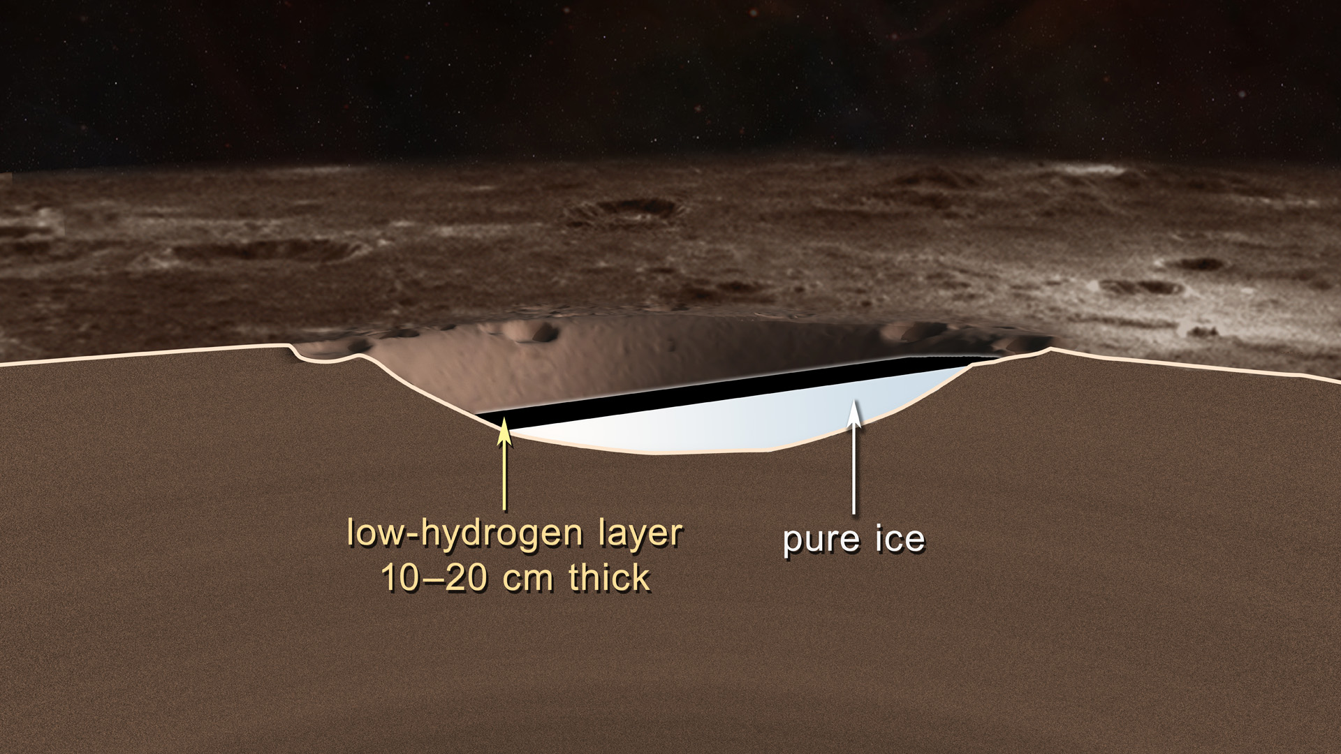
Image 3.4

MESSENGER neutron data show that Mercury’s north polar radar-bright deposits consist primarily of water ice. In most such areas, the water ice is covered by an insulating layer 10 to 20 cm thick.
Credit: NASA/Johns Hopkins University Applied Physics Laboratory/Carnegie Institution of Washington
Click on image to enlarge.
|
|
Presenter #4 |
Gregory A. Neumann, Mercury Laser Altimeter Instrument Scientist
NASA Goddard Space Flight Center, Greenbelt, Md
Video 4.1

The Mercury Laser Altimeter (MLA) is shown ranging to Mercury’s surface from orbit. In this animation, yellow flashes represent near-infrared laser pulses that can reflect off terrain in shadow as well as in sunlight. Using about as much power as a flashlight, the MLA instrument can range eight times a second to targets at distances as far as that from Washington, D.C., to Ottawa, Canada (~800 km), St. Louis, Missouri, or Orlando, Florida (~1200 km). The laser pulse returns from the surface in less than one hundredth of a second. This time interval can be measured to a precision equivalent to a hand’s breadth uncertainly in distance. Measurements are assembled from individual profiles to produce a terrain model such as the one shown here.
Credit: Scientific Visualization Studio, NASA Goddard Space Flight Center.
Click on image to watch video.
|
|
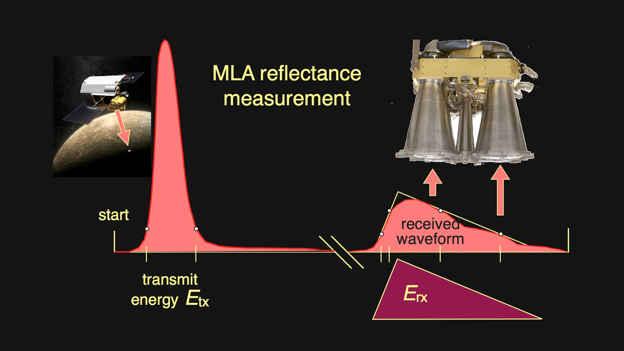
Image 4.2

An illustration of how MLA measures surface reflectance. The red curve shows (left) the waveform of a laser pulse transmitted to Mercury and (right) the detected pulse returned from a small area on the surface. The receiver telescopes detect at most a few hundred photons, and the pulse waveform is widened and distorted by the surface. The threshold-crossing times of the received pulse are measured at two discriminator voltages, a low threshold for maximum sensitivity, and when possible at a threshold approximately twice as high to give four sample points of the received pulse waveform. For a given distance, the reflectance is proportional to the ratio of the area of the received pulse to the integrated area of the transmitted pulse. The higher-threshold detection is possible only when the measurement is made at relatively low altitudes and with near-nadir incidence (<30° from the vertical), so as to produce a sufficiently strong return.
Credit: NASA Goddard Space Flight Center.
Click on image to enlarge.
|
|
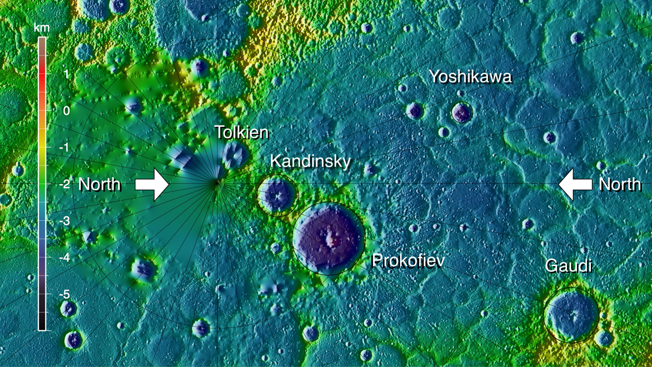
Image 4.3

Topography of a portion of Mercury from 75° N northward to the pole, in shaded relief and color-coded by elevation. The map is centered at 85°N on the 110-km-diameter crater Prokofiev, whose interior lies more than 5 km below the topographic datum. The north pole lies to the left of and below the smaller craters Tolkien and Kandinsky. Because of the inclination of MESSENGER’s orbit, ranging measurements poleward of 83-84°N require spacecraft maneuvers and oblique viewing. Most of the area north of these latitudes has been sparsely covered by MLA to date and is either seldom illuminated by sunlight or lies in permanent shadow.
Credit: NASA/Johns Hopkins University Applied Physics Laboratory/Carnegie Institution of Washington
Click on image to enlarge.
|
|
Image 4.4

Animation of the illumination of the topography from Image 4.3, showing the small proportion of sunlight that reaches the Prokofiev crater floor and rim. The north-facing portions of the rim and interior remain in perpetual shadow, as do those of numerous other craters. The movie simulates approximately one half of a Mercury solar day (176 Earth days) and uses the digital terrain model derived from MLA measurements. Contrast has been enhanced for television display.
Credit: NASA Goddard Space Flight Center/Massachusetts Institute of Technology/Johns Hopkins University Applied Physics Laboratory/Carnegie Institution of Washington.
Click on image to watch video.
|
|
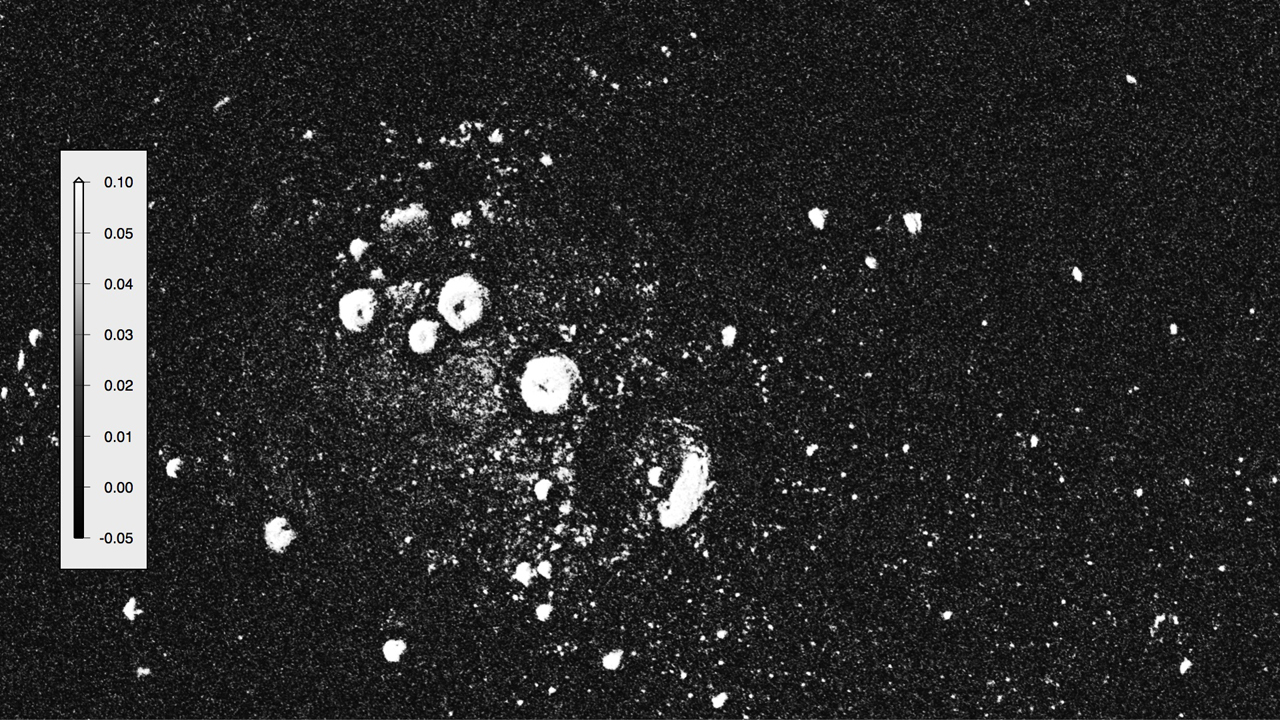
Image 4.5

A portion of the Arecibo radar image of Mercury’s north polar region that corresponds to the area of Image 4.3. Areas for which the radar cross-section exceeds 0.05 per unit area, believed to contain deposits with near-surface water ice, show as bright in this image.
Credit: National Astronomy and Ionosphere Center, Arecibo Observatory
Click on image to enlarge.
|
|
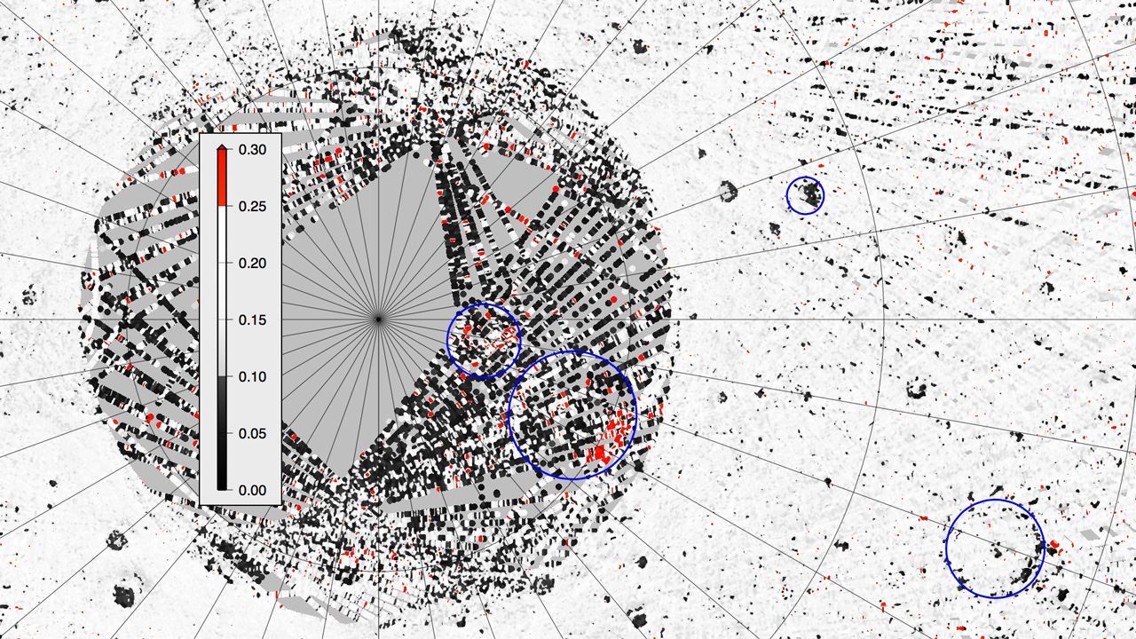
Image 4.6

Surface reflectance (relative to perfect Lambertian scattering) measured by MLA from profiles taken at incidence angles less than 30° from nadir. The orange/red areas are those with more than 50% higher reflectance than the regional average, consistent with surface exposures of water ice. Dark areas contain material of unusually low reflectance, about half the typical reflectance of Mercury. The dark areas are believed to be an insulating material that is stable to somewhat higher temperatures than water ice and protects the underlying ice deposits from thermal loss. The values are nearest-neighbor averages. Areas having no data within 2 km are shaded gray.
Credit: NASA/Johns Hopkins University Applied Physics Laboratory/Carnegie Institution of Washington
Click on image to enlarge.
|
|
Image 4.7

Montage of MLA topography, solar illumination from topography (selected for maximum illumination of Prokofiev), radar cross-section (inverted scale), and MLA reflectance at 1064 nm. The high optical reflectances on the north-facing interior of Prokofiev, and the close correspondence of MLA-dark and -bright regions with radar-bright areas and models of surface temperature (discussed next), indicate that the optically bright areas likely coincide with surface exposures of water ice. Optically dark surfaces in other radar-bright areas indicate a surficial layer of darker compounds.
Credit: NASA/Johns Hopkins University Applied Physics Laboratory/Carnegie Institution of Washington
Click on image to enlarge.
|
|
Presenter #5 |
David A. Paige, MESSENGER Participating Scientist
University of California, Los Angeles, Calif.
>
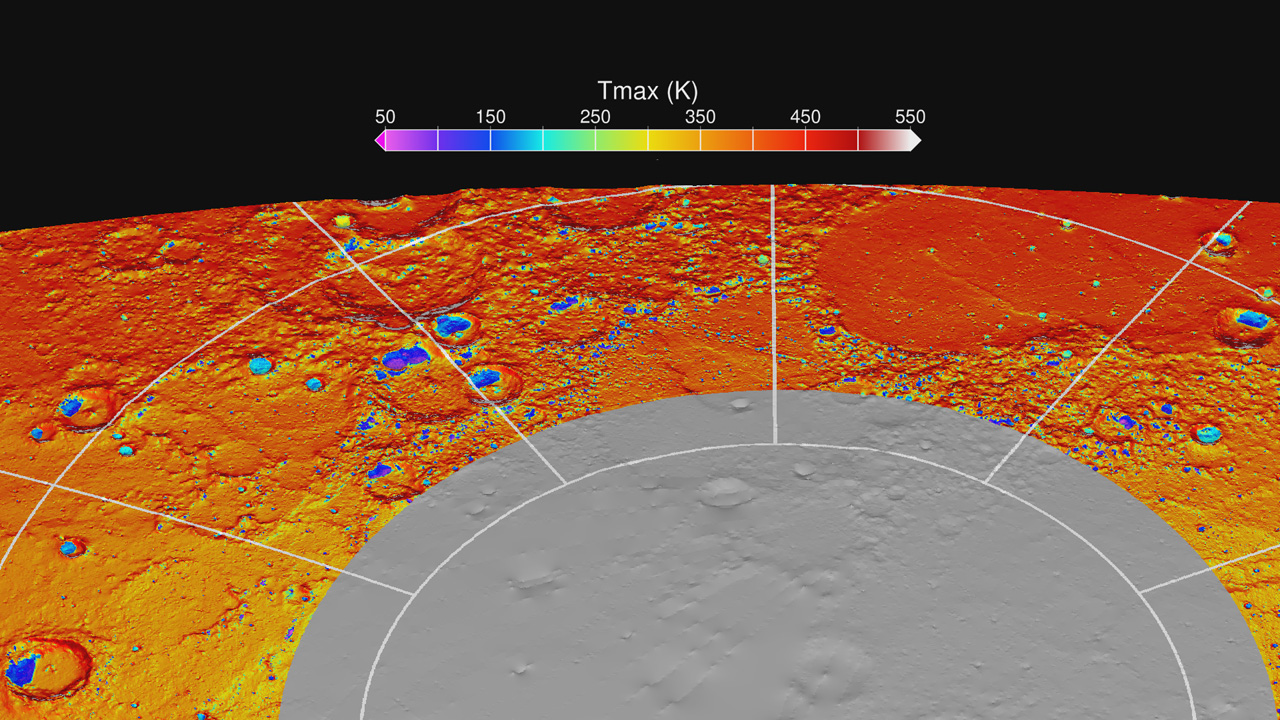
Image 5.1

Map of the maximum surface temperature reached over a two-year period over the north polar region of Mercury. This detailed thermal map of Mercury, and others that display additional thermal parameters, are the first to have been calculated from measurements of Mercury’s topography by the MESSENGER MLA instrument. Mercury displays the most extreme range of surface temperatures of any body in the solar system. Regions that receive direct sunlight at the equator reach maximum temperatures of 700 K (800° F), whereas regions in permanent shadow in high-latitude craters can drop below 50 K (-370° F). In this view from above Mercury's north pole, there are numerous craters with poleward-facing slopes on which the annual maximum temperature is less than 100 K (-280° F). At these temperatures, water ice is thermally stable over billion-year timescales.
Credit: NASA/UCLA/Johns Hopkins University Applied Physics Laboratory/Carnegie Institution of Washington
Click on image to enlarge.
|
|
Image 5.2

A map of "permafrost" on Mercury showing the calculated depths below the surface at which water ice is predicted to be thermally stable. The grey areas are regions that are too warm at all depths for stable water ice. The colored regions are sufficiently cold for subsurface ice to be stable, and the white regions are sufficiently cold exposed surface ice to be stable. The thermal model results predict the presence of surface and subsurface water ice at the same locations where they are observed by Earth-based radar and MLA observations.
Credit: NASA/UCLA/Johns Hopkins University Applied Physics Laboratory/Carnegie Institution of Washington
Click on image to enlarge.
|
|
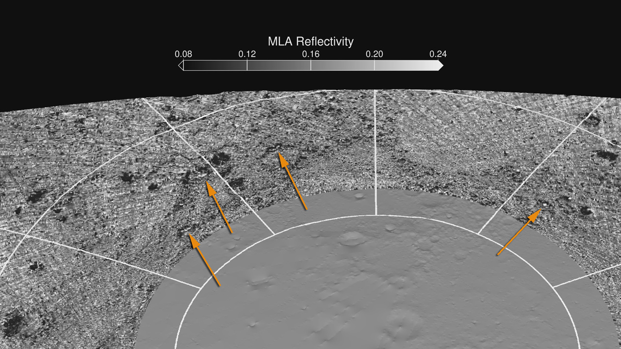
Image 5.3

Map of MLA reflectivity showing isolated areas of brighter and darker reflectance in areas of permanently shadow. Many of the brighter areas detected by MLA (as indicated by the arrows) are in unusually cold regions where surface water ice is predicted, as shown in Figure 2. In some cases, the dark regions are somewhat larger than the areas predicted to have thermally stable water ice.
Credit: NASA/UCLA/Johns Hopkins University Applied Physics Laboratory/Carnegie Institution of Washington
Click on image to enlarge.
|
|
| Image 5.4
A series of diagrams illustrating the formation of Mercury's polar ice deposits.
Image 5.4a

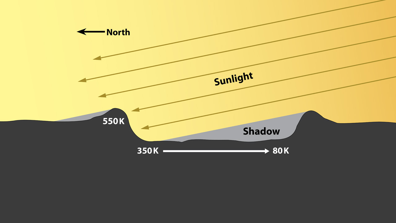
a) A high-latitude impact crater illuminated by the angled rays of the Sun creates a region of very warm temperatures on the illuminated rim, lower temperatures on the illuminated floor of the crater, and extremely cold temperatures in regions of permanent shadow.
Image 5.4b
 b) A comet or water-rich asteroid that also contains organic compounds impacts Mercury. b) A comet or water-rich asteroid that also contains organic compounds impacts Mercury.
Image 5.4c

c) The water and organic compounds are spread over a wide geographic region, and a small fraction of both compounds migrate to the poles where they can become cold-trapped as ices.
Image 5.4d

d) Over time, the water ice in the warmer regions vaporizes, leaving behind the more stable organic impurities at the surface.
Image 5.4e

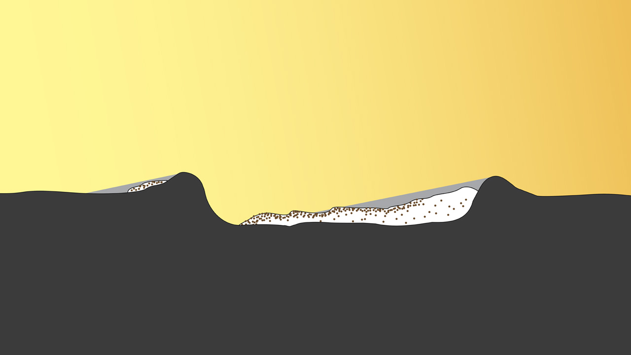
e) The ice retreats further to a stable long-term configuration. In the coldest areas, water ice remains on the surface. In the warmer areas, the ice is covered by an ice-free surface layer that is rich in organic impurities that have been darkened by exposure to Mercury's space environment.
Credit: NASA/UCLA/Johns Hopkins University Applied Physics Laboratory/Carnegie Institution of Washington
Click on image to enlarge.
|
|
The NASA MESSENGER News Conference will take place on Thursday, November 29, 2012, at 2 p.m. EST. Reporters may ask questions from participating NASA locations. The briefing also will be streamed live on NASA's Web site at: http://www.nasa.gov.